AlexNet deep dive: layer math, later architectures and PyTorch code
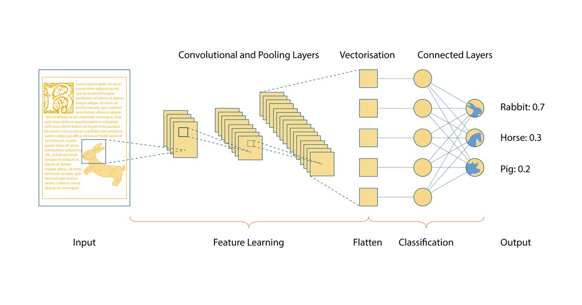
Illustrative image: A convolutional neural network: an input image passes through convolution and pooling layers to a classification output; illustrative of the deep learning approach AlexNet popularised. Image: Irisbox, CC BY 4.0, via Wikimedia Commons.
1. Layer-by-Layer Mathematical Breakdown
To compute the spatial output dimensions of any convolutional or pooling layer, AlexNet uses the standard formula:
Output Size = ⌊ (Input Size − Kernel Size + 2 × Padding) / Stride ⌋ + 1
(Note: In the original 2012 paper, the input dimension was written as 224 × 224 × 3 due to a slight typo; the exact arithmetic requires an input of 227 × 227 × 3 to yield the 55 × 55 output in Layer 1).
| Layer | Type | Input Shape | Filter / Kernel | Stride | Padding | Output Shape | Learned Parameters |
|---|---|---|---|---|---|---|---|
| Input | Image | 227 × 227 × 3 | — | — | — | 227 × 227 × 3 | 0 |
| Conv1 | Convolution + ReLU | 227 × 227 × 3 | 96 × (11 × 11 × 3) | 4 | 0 | 55 × 55 × 96 | 34,944 |
| Pool1 | Max Pooling | 55 × 55 × 96 | 3 × 3 | 2 | 0 | 27 × 27 × 96 | 0 |
| Conv2 | Convolution + ReLU | 27 × 27 × 96 | 256 × (5 × 5 × 96) | 1 | 2 | 27 × 27 × 256 | 614,656 |
| Pool2 | Max Pooling | 27 × 27 × 256 | 3 × 3 | 2 | 0 | 13 × 13 × 256 | 0 |
| Conv3 | Convolution + ReLU | 13 × 13 × 256 | 384 × (3 × 3 × 256) | 1 | 1 | 13 × 13 × 384 | 885,120 |
| Conv4 | Convolution + ReLU | 13 × 13 × 384 | 384 × (3 × 3 × 384) | 1 | 1 | 13 × 13 × 384 | 1,327,488 |
| Conv5 | Convolution + ReLU | 13 × 13 × 384 | 256 × (3 × 3 × 384) | 1 | 1 | 13 × 13 × 256 | 884,992 |
| Pool3 | Max Pooling | 13 × 13 × 256 | 3 × 3 | 2 | 0 | 6 × 6 × 256 | 0 |
| Flatten | Reshape | 6 × 6 × 256 | — | — | — | 9,216 | 0 |
| FC6 | Fully Connected + ReLU | 9,216 | 9,216 × 4,096 | — | — | 4,096 | 37,752,832 |
| FC7 | Fully Connected + ReLU | 4,096 | 4,096 × 4,096 | — | — | 4,096 | 16,781,312 |
| FC8 | Fully Connected + Softmax | 4,096 | 4,096 × 1,000 | — | — | 1,000 | 4,097,000 |
- Total Parameters: 62,378,344 (~62.4 million). Over 93% of these parameters sit inside the final three fully connected layers (FC6, FC7, FC8).
- Local Response Normalization (LRN): Originally applied after Conv1 and Conv2, LRN normalized neuron activity across neighboring channels. Modern implementations almost always replace LRN with Batch Normalization or omit it entirely.
2. Evolution: AlexNet vs. Later Architectures
Each major architecture after 2012 solved a specific bottleneck exposed by AlexNet.
| Feature | AlexNet (2012) | VGG-16 (2014) | ResNet-50 (2015) | Vision Transformer / ViT (2020) |
|---|---|---|---|---|
| Core Mechanism | Convolutions with large initial filters | Deep stacks of uniform small convolutions | Residual skip connections + BatchNorm | Self-attention over image patches |
| Depth (Learned Layers) | 8 | 16 | 50 | 12 to 32+ transformer blocks |
| Filter / Patch Size | 11×11, 5×5, 3×3 | Exclusively 3×3 | 7×7 stem, then 1×1 and 3×3 | 16×16 pixel patches (no convolutions) |
| Parameters | ~62.4 Million | ~138 Million | ~25.6 Million | ~86 Million (ViT-Base) |
| ImageNet Top-5 Error | 15.3% | 7.3% | 3.57% | < 1.5% (with pre-training) |
| Key Innovation | Proved deep CNNs + ReLU + GPUs scale | Showed stacked 3×3 filters match large receptive fields with fewer parameters | Solved vanishing gradients via identity shortcuts, allowing 100+ layers | Removed spatial inductive bias; treats images as sequences of tokens |
- Why VGG replaced large filters: Two stacked 3×3 filters cover the exact same receptive field as one 5×5 filter, and three stacked 3×3 filters cover an 11×11 area—while introducing more ReLU non-linearities and using far fewer parameters.
- Why ResNet reduced parameter bloat: ResNet replaced AlexNet's massive fully connected layers (FC6 and FC7) with Global Average Pooling, slashing parameter counts by more than half while jumping from 8 layers to 50+ layers.
- How ViT changed the paradigm: Vision Transformers abandoned convolutions entirely, splitting images into flat patches and applying the same Transformer attention mechanism used in Large Language Models.
3. Modern PyTorch Implementation
Below is a clean, self-contained PyTorch implementation of AlexNet using modern best practices (such as standard 224 × 224 inputs with adjusted padding on Conv1, and Adaptive Average Pooling so the model accepts flexible input resolutions).
import torch
import torch.nn as nn
import torch.optim as optim

class AlexNet(nn.Module):
    def __init__(self, num_classes: int = 1000, dropout: float = 0.5):
        super().__init__()

        # Feature extractor (5 Convolutional layers)
        self.features = nn.Sequential(
            # Conv1: 224x224x3 -> 55x55x64 (Modern PyTorch standard uses 64 filters & pad=2)
            nn.Conv2d(3, 64, kernel_size=11, stride=4, padding=2),
            nn.ReLU(inplace=True),
            nn.MaxPool2d(kernel_size=3, stride=2),

            # Conv2: 27x27x64 -> 27x27x192
            nn.Conv2d(64, 192, kernel_size=5, padding=2),
            nn.ReLU(inplace=True),
            nn.MaxPool2d(kernel_size=3, stride=2),

            # Conv3: 13x13x192 -> 13x13x384
            nn.Conv2d(192, 384, kernel_size=3, padding=1),
            nn.ReLU(inplace=True),

            # Conv4: 13x13x384 -> 13x13x256
            nn.Conv2d(384, 256, kernel_size=3, padding=1),
            nn.ReLU(inplace=True),

            # Conv5: 13x13x256 -> 13x13x256 -> Pool -> 6x6x256
            nn.Conv2d(256, 256, kernel_size=3, padding=1),
            nn.ReLU(inplace=True),
            nn.MaxPool2d(kernel_size=3, stride=2),
        )

        # Ensures output is always 6x6 regardless of slight input image size variations
        self.avgpool = nn.AdaptiveAvgPool2d((6, 6))

        # Classifier (3 Fully Connected layers)
        self.classifier = nn.Sequential(
            nn.Dropout(p=dropout),
            nn.Linear(256 * 6 * 6, 4096),
            nn.ReLU(inplace=True),

            nn.Dropout(p=dropout),
            nn.Linear(4096, 4096),
            nn.ReLU(inplace=True),

            nn.Linear(4096, num_classes),
        )

    def forward(self, x: torch.Tensor) -> torch.Tensor:
        x = self.features(x)
        x = self.avgpool(x)
        x = torch.flatten(x, 1)
        x = self.classifier(x)
        return x


# --- Quick Training Loop Example ---
if __name__ == "__main__":
    device = torch.device("cuda" if torch.cuda.is_available() else "cpu")

    # Instantiate for a 10-class dataset (e.g., CIFAR-10 upscaled or Imagenette)
    model = AlexNet(num_classes=10).to(device)
    criterion = nn.CrossEntropyLoss()
    optimizer = optim.AdamW(model.parameters(), lr=1e-4, weight_decay=1e-2)

    # Dummy batch: 8 RGB images of size 224x224
    dummy_images = torch.randn(8, 3, 224, 224, device=device)
    dummy_labels = torch.randint(0, 10, (8,), device=device)

    # Single forward + backward training step
    model.train()
    optimizer.zero_grad()
    outputs = model(dummy_images)
    loss = criterion(outputs, dummy_labels)
    loss.backward()
    optimizer.step()

print(f"Device: {device} | Output shape: {outputs.shape} | Step loss: {loss.item():.4f}")- Modern Adjustments in Code: Standard torchvision.models.alexnet uses slightly streamlined channel counts (64, 192, 384, 256, 256) rather than the original paper's split-GPU counts (96, 256, 384, 384, 256), and uses AdamW instead of SGD with momentum for faster convergence on smaller datasets.
- Transfer Learning Shortcut: If you want to fine-tune a pre-trained AlexNet rather than training from scratch, you can load it directly via torchvision.models.alexnet(weights="DEFAULT") and replace model.classifier[6] = nn.Linear(4096, your_num_classes).